|
|
|
 GitHub पर सोर्स देखना GitHub पर सोर्स देखना
|
|
इस कोडलैब में, पैरामीटर-एफ़िशिएंट ट्यूनिंग (पीईटी) का इस्तेमाल करके, पसंद के मुताबिक टेक्स्ट क्लासिफ़ायर बनाने का तरीका बताया गया है. पूरे मॉडल को फ़ाइन-ट्यून करने के बजाय, पीईटी के तरीके सिर्फ़ कुछ पैरामीटर अपडेट करते हैं. इससे मॉडल को ट्रेन करना आसान और तेज़ हो जाता है. इससे मॉडल को कम ट्रेनिंग डेटा के साथ भी नए व्यवहारों को सीखना आसान हो जाता है. इस तरीके के बारे में ज़्यादा जानकारी सभी के लिए एजाइल टेक्स्ट क्लासिफ़ायर की ओर लेख में दी गई है. इसमें बताया गया है कि इन तकनीकों को सुरक्षा से जुड़े अलग-अलग टास्क पर कैसे लागू किया जा सकता है और सिर्फ़ कुछ सौ ट्रेनिंग उदाहरणों की मदद से, बेहतरीन परफ़ॉर्मेंस कैसे हासिल की जा सकती है.
इस कोडलैब में, LoRA पीईटी तरीके और छोटे Gemma मॉडल (gemma_instruct_2b_en) का इस्तेमाल किया गया है, क्योंकि इसे तेज़ी से और ज़्यादा बेहतर तरीके से चलाया जा सकता है. इस कोलब में, डेटा डालने, एलएलएम के लिए उसे फ़ॉर्मैट करने, LoRA वेट को ट्रेन करने, और फिर नतीजों का आकलन करने का तरीका बताया गया है. इस कोडलैब में, ETHOS डेटासेट का इस्तेमाल किया गया है. यह डेटासेट, YouTube और Reddit पर की गई टिप्पणियों से तैयार किया गया है. यह सार्वजनिक तौर पर उपलब्ध है और इसका इस्तेमाल, नफ़रत फैलाने वाली भाषा का पता लगाने के लिए किया जाता है.
सिर्फ़ 200 उदाहरणों (डेटासेट का 1/4) पर ट्रेनिंग देने पर, यह एल्गोरिदम F1: 0.80 और
आरओसी-एयूसी: 0.78 हासिल करता है. यह वैल्यू, लीडरबोर्ड पर मौजूद, फ़िलहाल सबसे बेहतर एल्गोरिदम से थोड़ी ज़्यादा है. यह वैल्यू, 15 फ़रवरी, 2024 को लिखे जाने के समय की है. जब इसे 800 उदाहरणों पर ट्रेन किया जाता है, तो यह 83.74 का एफ़1 स्कोर और 88.17 का आरओसी-एयूसी स्कोर हासिल करता है. आम तौर पर, gemma_instruct_7b_en जैसे बड़े मॉडल बेहतर परफ़ॉर्म करते हैं. हालांकि, इनकी ट्रेनिंग और लागू करने की लागत भी ज़्यादा होती है.
ट्रिगर से जुड़ी चेतावनी: इस कोडलैब में, नफ़रत फैलाने वाली भाषा का पता लगाने के लिए, सुरक्षा क्लासिफ़ायर डेवलप किया जाता है. इसलिए, नतीजों के उदाहरणों और उनके आकलन में कुछ भयानक भाषा का इस्तेमाल किया गया है.
इंस्टॉल और सेटअप करना
इस कोडलैब के लिए, आपको Gemma मॉडल डाउनलोड करने के लिए, keras (3), keras-nlp (0.8.0) का नया वर्शन और Kaggle खाता चाहिए.
import kagglehub

kagglehub.login()
pip install -q -U keras-nlppip install -q -U keras
import os

os.environ["KERAS_BACKEND"] = "tensorflow"
ETHOS डेटासेट लोड करना
इस सेक्शन में, आपको वह डेटासेट लोड करना होगा जिस पर हमारे क्लासिफ़ायर को ट्रेनिंग देनी है. साथ ही, उसे ट्रेन और टेस्ट सेट में प्री-प्रोसेस करना होगा. आपको लोकप्रिय रिसर्च डेटासेट ETHOS का इस्तेमाल करना होगा. इसे सोशल मीडिया पर नफ़रत फैलाने वाली भाषा का पता लगाने के लिए इकट्ठा किया गया था. डेटासेट इकट्ठा करने के तरीके के बारे में ज़्यादा जानने के लिए, ETHOS: नफ़रत फैलाने वाली भाषा का पता लगाने वाला ऑनलाइन डेटासेट पेपर पढ़ें.
import pandas as pd

gh_root = 'https://raw.githubusercontent.com'
gh_repo = 'intelligence-csd-auth-gr/Ethos-Hate-Speech-Dataset'
gh_path = 'master/ethos/ethos_data/Ethos_Dataset_Binary.csv'
data_url = f'{gh_root}/{gh_repo}/{gh_path}'

df = pd.read_csv(data_url, delimiter=';')
df['hateful'] = (df['isHate'] >= df['isHate'].median()).astype(int)

# Shuffle the dataset.
df = df.sample(frac=1, random_state=32)

# Split into train and test.
df_train, df_test = df[:800],  df[800:]

# Display a sample of the data.
df.head(5)[['hateful', 'comment']]
मॉडल डाउनलोड करना और उसे इंस्टैंशिएट करना
दस्तावेज़ में बताए गए तरीके से, Gemma मॉडल का इस्तेमाल कई तरीकों से आसानी से किया जा सकता है. Keras का इस्तेमाल करने के लिए, आपको यह तरीका अपनाना होगा:
import keras
import keras_nlp

# For reproducibility purposes.
keras.utils.set_random_seed(1234)

# Download the model from Kaggle using Keras.
model = keras_nlp.models.GemmaCausalLM.from_preset('gemma_instruct_2b_en')

# Set the sequence length to a small enough value to fit in memory in Colab.
model.preprocessor.sequence_length = 128
model.generate('Question: what is the capital of France? ', max_length=32)
टेक्स्ट की प्री-प्रोसेसिंग और सेपरेटर टोकन
मॉडल को हमारे इंटेंट को बेहतर तरीके से समझने में मदद करने के लिए, टेक्स्ट को पहले से प्रोसेस किया जा सकता है और अलग करने वाले टोकन का इस्तेमाल किया जा सकता है. इससे, मॉडल के लिए ऐसा टेक्स्ट जनरेट करने की संभावना कम हो जाती है जो सही फ़ॉर्मैट में न हो. उदाहरण के लिए, इस तरह का प्रॉम्प्ट लिखकर, मॉडल से सेंटीमेंट कैटगरी का अनुरोध किया जा सकता है:
Classify the following text into one of the following classes:[Positive,Negative]

Text: you look very nice today
Classification:
इस मामले में, हो सकता है कि मॉडल आपके हिसाब से नतीजे दिखाए या न दिखाए. उदाहरण के लिए, अगर टेक्स्ट में न्यू लाइन वर्ण हैं, तो मॉडल की परफ़ॉर्मेंस पर इसका बुरा असर पड़ सकता है. सेपरेटर टोक़न का इस्तेमाल करना, एक बेहतर तरीका है. इसके बाद, प्रॉम्प्ट इस तरह दिखेगा:
Classify the following text into one of the following classes:[Positive,Negative]
<separator>
Text: you look very nice today
<separator>
Prediction:
टेक्स्ट को पहले से प्रोसेस करने वाले फ़ंक्शन का इस्तेमाल करके, इसे अलग किया जा सकता है:
def preprocess_text(
    text: str,
    labels: list[str],
    instructions: str,
    separator: str,
) -> str:
  prompt = f'{instructions}:[{",".join(labels)}]'
  return separator.join([prompt, f'Text:{text}', 'Prediction:'])
अब, अगर पहले की तरह ही प्रॉम्प्ट और टेक्स्ट का इस्तेमाल करके फ़ंक्शन को चलाया जाता है, तो आपको वही आउटपुट मिलना चाहिए:
text = 'you look very nice today'

prompt = preprocess_text(
    text=text,
    labels=['Positive', 'Negative'],
    instructions='Classify the following text into one of the following classes',
    separator='\n<separator>\n',
)

print(prompt)
Classify the following text into one of the following classes:[Positive,Negative]
<separator>
Text:you look very nice today
<separator>
Prediction:
आउटपुट पोस्ट-प्रोसेसिंग
मॉडल के आउटपुट, अलग-अलग संभावनाओं वाले टोकन होते हैं. आम तौर पर, टेक्स्ट जनरेट करने के लिए, सबसे संभावित कुछ टोक़न में से किसी एक को चुना जाता है. इसके बाद, उससे वाक्य, पैराग्राफ़ या पूरे दस्तावेज़ बनाए जाते हैं. हालांकि, कैटगरी तय करने के लिए, यह ज़रूरी है कि मॉडल को लगता हो कि Positive की संभावना Negative से ज़्यादा है या इसके उलट.
आपने पहले जिस मॉडल को इंस्टैंशिएट किया था उसके आउटपुट को, अगला टोकन Positive या Negative है या नहीं, इसकी अलग-अलग संभावनाओं के हिसाब से प्रोसेस करने का तरीका यहां बताया गया है:
import numpy as np


def compute_output_probability(
    model: keras_nlp.models.GemmaCausalLM,
    prompt: str,
    target_classes: list[str],
) -> dict[str, float]:
  # Shorthands.
  preprocessor = model.preprocessor
  tokenizer = preprocessor.tokenizer

  # NOTE: If a token is not found, it will be considered same as "<unk>".
  token_unk = tokenizer.token_to_id('<unk>')

  # Identify the token indices, which is the same as the ID for this tokenizer.
  token_ids = [tokenizer.token_to_id(word) for word in target_classes]

  # Throw an error if one of the classes maps to a token outside the vocabulary.
  if any(token_id == token_unk for token_id in token_ids):
    raise ValueError('One of the target classes is not in the vocabulary.')

  # Preprocess the prompt in a single batch. This is done one sample at a time
  # for illustration purposes, but it would be more efficient to batch prompts.
  preprocessed = model.preprocessor.generate_preprocess([prompt])

  # Identify output token offset.
  padding_mask = preprocessed["padding_mask"]
  token_offset = keras.ops.sum(padding_mask) - 1

  # Score outputs, extract only the next token's logits.
  vocab_logits = model.score(
      token_ids=preprocessed["token_ids"],
      padding_mask=padding_mask,
  )[0][token_offset]

  # Compute the relative probability of each of the requested tokens.
  token_logits = [vocab_logits[ix] for ix in token_ids]
  logits_tensor = keras.ops.convert_to_tensor(token_logits)
  probabilities = keras.activations.softmax(logits_tensor)

  return dict(zip(target_classes, probabilities.numpy()))
उस फ़ंक्शन की जांच करने के लिए, उसे पहले बनाए गए प्रॉम्प्ट के साथ चलाएं:
compute_output_probability(
    model=model,
    prompt=prompt,
    target_classes=['Positive', 'Negative'],
)
{'Positive': 0.99994016, 'Negative': 5.984089e-05}
इसे क्लासिफ़ायर के तौर पर रैप करना
इस्तेमाल करने में आसानी के लिए, आपने अभी जो फ़ंक्शन बनाए हैं उन्हें एक साथ रैप करके, sklearn जैसे क्लासिफ़ायर में डाला जा सकता है. इसमें predict() और predict_score() जैसे आसान और जाने-पहचाने फ़ंक्शन शामिल होते हैं.
import dataclasses


@dataclasses.dataclass(frozen=True)
class AgileClassifier:
  """Agile classifier to be wrapped around a LLM."""

  # The classes whose probability will be predicted.
  labels: tuple[str, ...]

  # Provide default instructions and control tokens, can be overridden by user.
  instructions: str = 'Classify the following text into one of the following classes'
  separator_token: str = '<separator>'
  end_of_text_token: str = '<eos>'

  def encode_for_prediction(self, x_text: str) -> str:
    return preprocess_text(
        text=x_text,
        labels=self.labels,
        instructions=self.instructions,
        separator=self.separator_token,
    )

  def encode_for_training(self, x_text: str, y: int) -> str:
    return ''.join([
        self.encode_for_prediction(x_text),
        self.labels[y],
        self.end_of_text_token,
    ])

  def predict_score(
      self,
      model: keras_nlp.models.GemmaCausalLM,
      x_text: str,
  ) -> list[float]:
    prompt = self.encode_for_prediction(x_text)
    token_probabilities = compute_output_probability(
        model=model,
        prompt=prompt,
        target_classes=self.labels,
    )
    return [token_probabilities[token] for token in self.labels]

  def predict(
      self,
      model: keras_nlp.models.GemmaCausalLM,
      x_eval: str,
  ) -> int:
    return np.argmax(self.predict_score(model, x_eval))

agile_classifier = AgileClassifier(labels=('Positive', 'Negative'))
मॉडल को बेहतर बनाना
LoRA का मतलब है, कम रैंक वाला अडैप्टेशन. यह फ़ाइन-ट्यून करने की एक तकनीक है. इसका इस्तेमाल, लार्ज लैंग्वेज मॉडल को बेहतर बनाने के लिए किया जा सकता है. इस बारे में ज़्यादा जानने के लिए, LoRA: Low-Rank Adaptation of Large Language Models पेपर पढ़ें.
Gemma को Keras में लागू करने पर, enable_lora() का एक तरीका मिलता है. इसका इस्तेमाल, बेहतर बनाने के लिए किया जा सकता है:
# Enable LoRA for the model and set the LoRA rank to 4.
model.backbone.enable_lora(rank=4)
LoRA को चालू करने के बाद, फ़ाइन-ट्यून करने की प्रोसेस शुरू की जा सकती है. Colab पर हर एपिसोड को पूरा होने में करीब पांच मिनट लगते हैं:
import tensorflow as tf

# Create dataset with preprocessed text + labels.
map_fn = lambda x: agile_classifier.encode_for_training(*x)
x_train = list(map(map_fn, df_train[['comment', 'hateful']].values))
ds_train = tf.data.Dataset.from_tensor_slices(x_train).batch(2)

# Compile the model using the Adam optimizer and appropriate loss function.
model.compile(
    loss=keras.losses.SparseCategoricalCrossentropy(from_logits=True),
    optimizer=keras.optimizers.Adam(learning_rate=0.0005),
    weighted_metrics=[keras.metrics.SparseCategoricalAccuracy()],
)

# Begin training.
model.fit(ds_train, epochs=4)
Epoch 1/4
400/400 ━━━━━━━━━━━━━━━━━━━━ 354s 703ms/step - loss: 1.1365 - sparse_categorical_accuracy: 0.5874
Epoch 2/4
400/400 ━━━━━━━━━━━━━━━━━━━━ 338s 716ms/step - loss: 0.7579 - sparse_categorical_accuracy: 0.6662
Epoch 3/4
400/400 ━━━━━━━━━━━━━━━━━━━━ 324s 721ms/step - loss: 0.6818 - sparse_categorical_accuracy: 0.6894
Epoch 4/4
400/400 ━━━━━━━━━━━━━━━━━━━━ 323s 725ms/step - loss: 0.5922 - sparse_categorical_accuracy: 0.7220
<keras.src.callbacks.history.History at 0x7eb7e369c490>
ज़्यादा एपिसोड के लिए ट्रेनिंग करने पर, नतीजे ज़्यादा सटीक होंगे. हालांकि, ऐसा तब तक होगा, जब तक ओवरफ़िटिंग नहीं होती.
नतीजों की जांच करना
अब आपके पास, हाल ही में ट्रेन किए गए एजाइल क्लासिफ़ायर के आउटपुट की जांच करने का विकल्प है. यह कोड, किसी टेक्स्ट के आधार पर क्लास का अनुमानित स्कोर दिखाएगा:
text = 'you look really nice today'
scores = agile_classifier.predict_score(model, text)
dict(zip(agile_classifier.labels, scores))
{'Positive': 0.99899644, 'Negative': 0.0010035498}
मॉडल का आकलन
आखिर में, आपको दो सामान्य मेट्रिक का इस्तेमाल करके, हमारे मॉडल की परफ़ॉर्मेंस का आकलन करना होगा. ये मेट्रिक हैं, F1 स्कोर और AUC-ROC. एफ़1 स्कोर, किसी क्लासिफ़िकेशन थ्रेशोल्ड पर प्रिसिज़न और रीकॉल के हार्मोनिक मीन का आकलन करके, फ़ॉल्स नेगेटिव और फ़ॉल्स पॉज़िटिव गड़बड़ियों को कैप्चर करता है. दूसरी ओर, AUC-ROC कई थ्रेशोल्ड में ट्रू पॉज़िटिव रेट और फ़ॉल्स पॉज़िटिव रेट के बीच के समझौते को कैप्चर करता है और इस कर्व के नीचे के हिस्से का हिसाब लगाता है.
y_true = df_test['hateful'].values
# Compute the scores (aka probabilities) for each of the labels.
y_score = [agile_classifier.predict_score(model, x) for x in df_test['comment']]
# The label with highest score is considered the predicted class.
y_pred = np.argmax(y_score, axis=1)
# Extract the probability of a comment being considered hateful.
y_prob = [x[agile_classifier.labels.index('Negative')] for x in y_score]
from sklearn.metrics import f1_score, roc_auc_score

print(f'F1: {f1_score(y_true, y_pred):.2f}')
print(f'AUC-ROC: {roc_auc_score(y_true, y_prob):.2f}')
F1: 0.84
AUC-ROC: 0.88
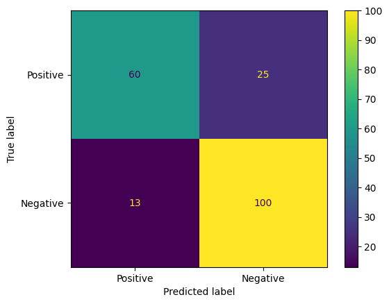
मॉडल के अनुमान का आकलन करने का एक और दिलचस्प तरीका, कन्फ़्यूज़न मैट्रिक है. कंफ़्यूज़न मैट्रिक, अलग-अलग तरह की गड़बड़ियों को विज़ुअल तौर पर दिखाएगी.
from sklearn.metrics import confusion_matrix, ConfusionMatrixDisplay

cm = confusion_matrix(y_true, y_pred)
ConfusionMatrixDisplay(
    confusion_matrix=cm,
    display_labels=agile_classifier.labels,
).plot()
<sklearn.metrics._plot.confusion_matrix.ConfusionMatrixDisplay at 0x7eb7e2d29ab0>
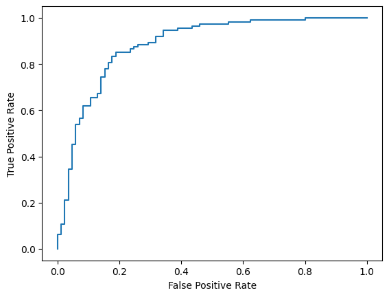
आखिर में, अलग-अलग स्कोरिंग थ्रेशोल्ड का इस्तेमाल करके, अनुमान से जुड़ी संभावित गड़बड़ियों के बारे में जानने के लिए आरओसी कर्व भी देखा जा सकता है.
from sklearn.metrics import RocCurveDisplay, roc_curve

fpr, tpr, _ = roc_curve(y_true, y_prob, pos_label=1)
RocCurveDisplay(fpr=fpr, tpr=tpr).plot()
<sklearn.metrics._plot.roc_curve.RocCurveDisplay at 0x7eb4d130ef20>
अन्य जानकारी
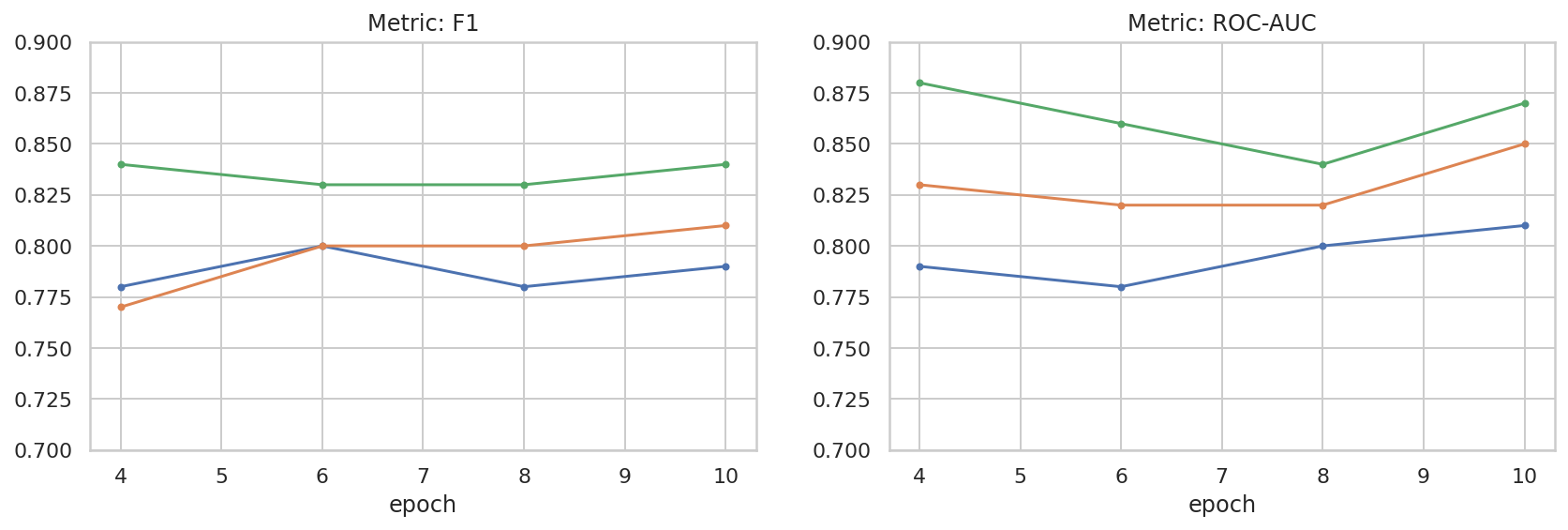
हमने डेटासेट के साइज़ और परफ़ॉर्मेंस के बीच के संबंध को बेहतर तरीके से समझने के लिए, हाइपर-पैरामीटर स्पेस का कुछ बुनियादी एक्सप्लोरेशन किया है. नीचे दिया गया प्लॉट देखें.
import matplotlib.pyplot as plt
import pandas as pd
import seaborn as sns

sns.set_theme(style="whitegrid")

results_f1 = pd.DataFrame([
    {'training_size': 800, 'epoch': 4, 'metric': 'f1', 'score': 0.84},
    {'training_size': 800, 'epoch': 6, 'metric': 'f1', 'score': 0.83},
    {'training_size': 800, 'epoch': 8, 'metric': 'f1', 'score': 0.83},
    {'training_size': 800, 'epoch': 10, 'metric': 'f1', 'score': 0.84},
    {'training_size': 400, 'epoch': 4, 'metric': 'f1', 'score': 0.77},
    {'training_size': 400, 'epoch': 6, 'metric': 'f1', 'score': 0.80},
    {'training_size': 400, 'epoch': 8, 'metric': 'f1', 'score': 0.80},
    {'training_size': 400, 'epoch': 10,'metric': 'f1', 'score': 0.81},
    {'training_size': 200, 'epoch': 4, 'metric': 'f1', 'score': 0.78},
    {'training_size': 200, 'epoch': 6, 'metric': 'f1', 'score': 0.80},
    {'training_size': 200, 'epoch': 8, 'metric': 'f1', 'score': 0.78},
    {'training_size': 200, 'epoch': 10, 'metric': 'f1', 'score': 0.79},
])

results_roc_auc = pd.DataFrame([
    {'training_size': 800, 'epoch': 4, 'metric': 'roc-auc', 'score': 0.88},
    {'training_size': 800, 'epoch': 6, 'metric': 'roc-auc', 'score': 0.86},
    {'training_size': 800, 'epoch': 8, 'metric': 'roc-auc', 'score': 0.84},
    {'training_size': 800, 'epoch': 10, 'metric': 'roc-auc', 'score': 0.87},
    {'training_size': 400, 'epoch': 4, 'metric': 'roc-auc', 'score': 0.83},
    {'training_size': 400, 'epoch': 6, 'metric': 'roc-auc', 'score': 0.82},
    {'training_size': 400, 'epoch': 8, 'metric': 'roc-auc', 'score': 0.82},
    {'training_size': 400, 'epoch': 10,'metric': 'roc-auc', 'score': 0.85},
    {'training_size': 200, 'epoch': 4, 'metric': 'roc-auc', 'score': 0.79},
    {'training_size': 200, 'epoch': 6, 'metric': 'roc-auc', 'score': 0.78},
    {'training_size': 200, 'epoch': 8, 'metric': 'roc-auc', 'score': 0.80},
    {'training_size': 200, 'epoch': 10, 'metric': 'roc-auc', 'score': 0.81},
])


plot_opts = dict(style='.-', ylim=(0.7, 0.9))
fig, (ax1, ax2) = plt.subplots(1, 2, figsize=(14, 4))
process_results_df = lambda df: df.set_index('epoch').groupby('training_size')['score']
process_results_df(results_f1).plot(title='Metric: F1', ax=ax1, **plot_opts)
process_results_df(results_roc_auc).plot(title='Metric: ROC-AUC', ax=ax2, **plot_opts)
fig.show()